COPY / PASTE HERE:

c(0,10^(1:7))

paste0(‘<=’,scales::comma(c(10^(1:7))))

Some of the datasets I deal with are lognormally distributed. Basically what this means is they follow the 80/20 rule where 80% of the sum of the values comes from the top 20% of the observations when sorted descending. There are a lot of observations with very low values relative to the range. Often I bucket things into bins for reporting based on log base-10 rule where we bucket “observations less than 10”, then observations less than 100 then 1,000 then 10,000 etc. This helps make large distributions more easily digestible and helps any observer quickly get a feel for the state of the data.

When I don’t have time to mess around with googling stuff I’ll write this out the way my brain says it. e.g. with ifelse() inside a mutate().

dataframe %<>%
  mutate(
    bucket = ifelse(
      n <= 10,'<=10'
      , n<= 100, '<= 100'
      , n <= 1000, '<= 1,000'
      ...
    )
  )

This obviously SUCKS. R is built for crap like this using stuff like the cut() function.

The problem with cut though is that I still found myself writing long statements with manual breaks. e.g.

dataframe %<>%
  mutate(
    bucket = cut(
      n
      , breaks=c(0,10,100,1e3,1e4,1e5,1e6,1e7,1e8)
      , labels=c('<= 10','<= 100','<= 1,000','<= 10,000','<= 100,000','<= 1,000,000','<= 10,000,000','<= 100,000,000')
    )
  )

That was better. But that obviously still sucks.

This type of binning in R is easy with R’s syntax 10^(1:n).

So let’s generate a lognormal distribution with some really high outliers.

impressions <- data.frame(rlnorm(n=100000, meanlog = log(100000), sdlog=log(5)))

names( impressions) <-'imps'

head( impressions)

##         imps
## 1   4900.182
## 2  55144.003
## 3 409891.498
## 4 163868.240
## 5  27864.676
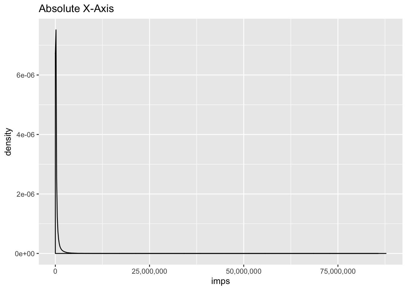
## 6 731740.292

You can see this is pretty heavily biased to the low end:

library( ggplot2)

ggplot( impressions, aes(x=imps)) +
  geom_density() +
  scale_x_continuous(labels=scales::comma) +
  labs(title = 'Absolute X-Axis')

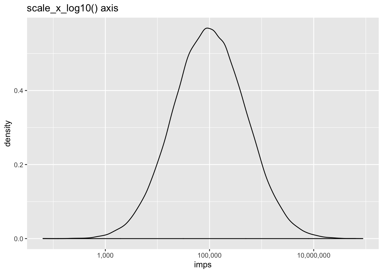
ggplot(impressions, aes(x=imps)) +
  geom_density() +
  scale_x_log10(labels=scales::comma) +
  labs(title = 'scale_x_log10() axis')

So let’s bin this up into logarithmic bins.

library( dplyr)
library( magrittr)
library( scales)

 
impressions %<>%
  mutate(
    bucket = cut(
      imps
      , breaks = c(0,10^(1:8))
      , labels = c(paste0('<= ',scales::comma(c(10^(1:8)))))
    )
  )

head(impressions)

##         imps       bucket
## 1   4900.182    <= 10,000
## 2  55144.003   <= 100,000
## 3 409891.498 <= 1,000,000
## 4 163868.240 <= 1,000,000
## 5  27864.676   <= 100,000
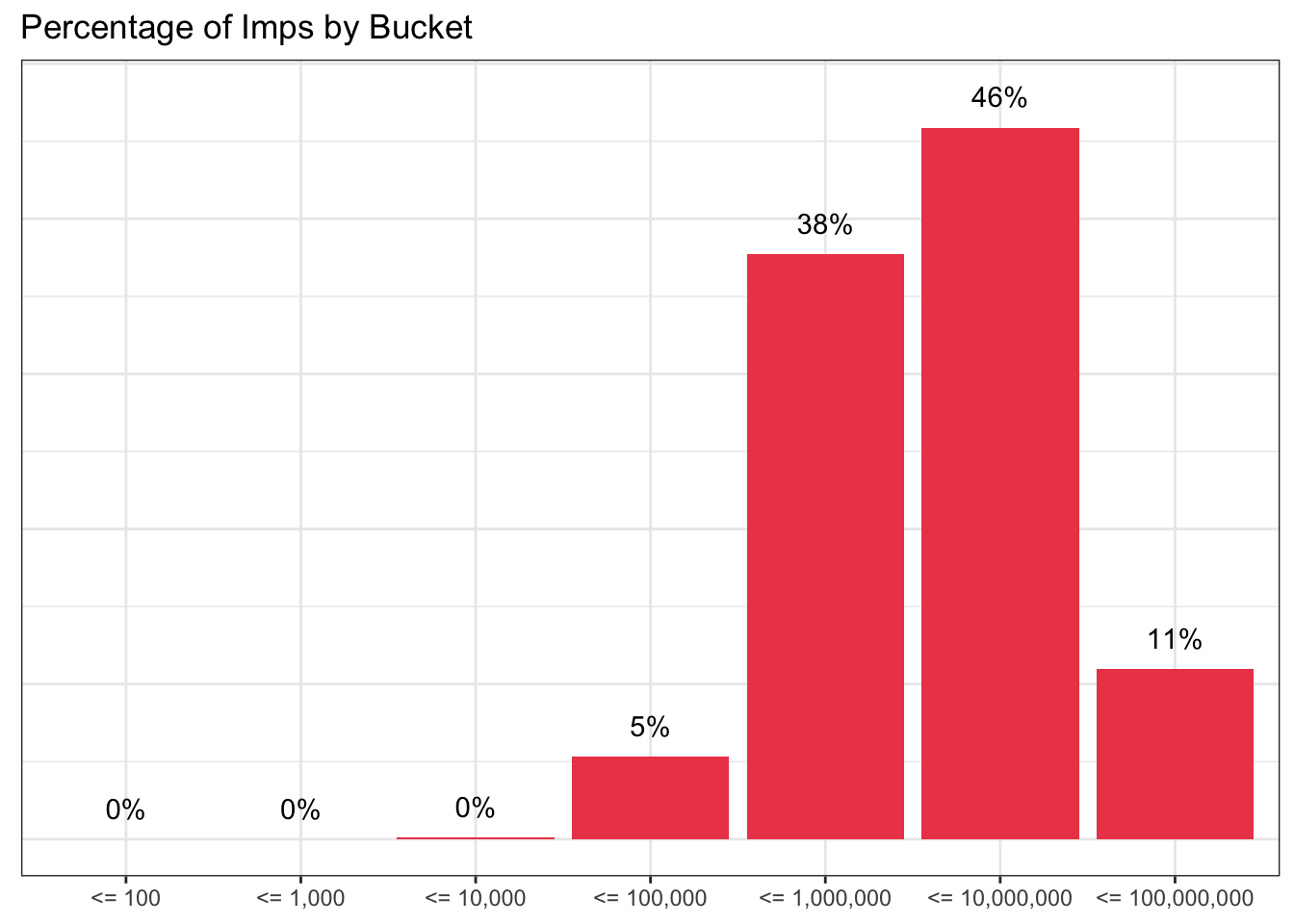
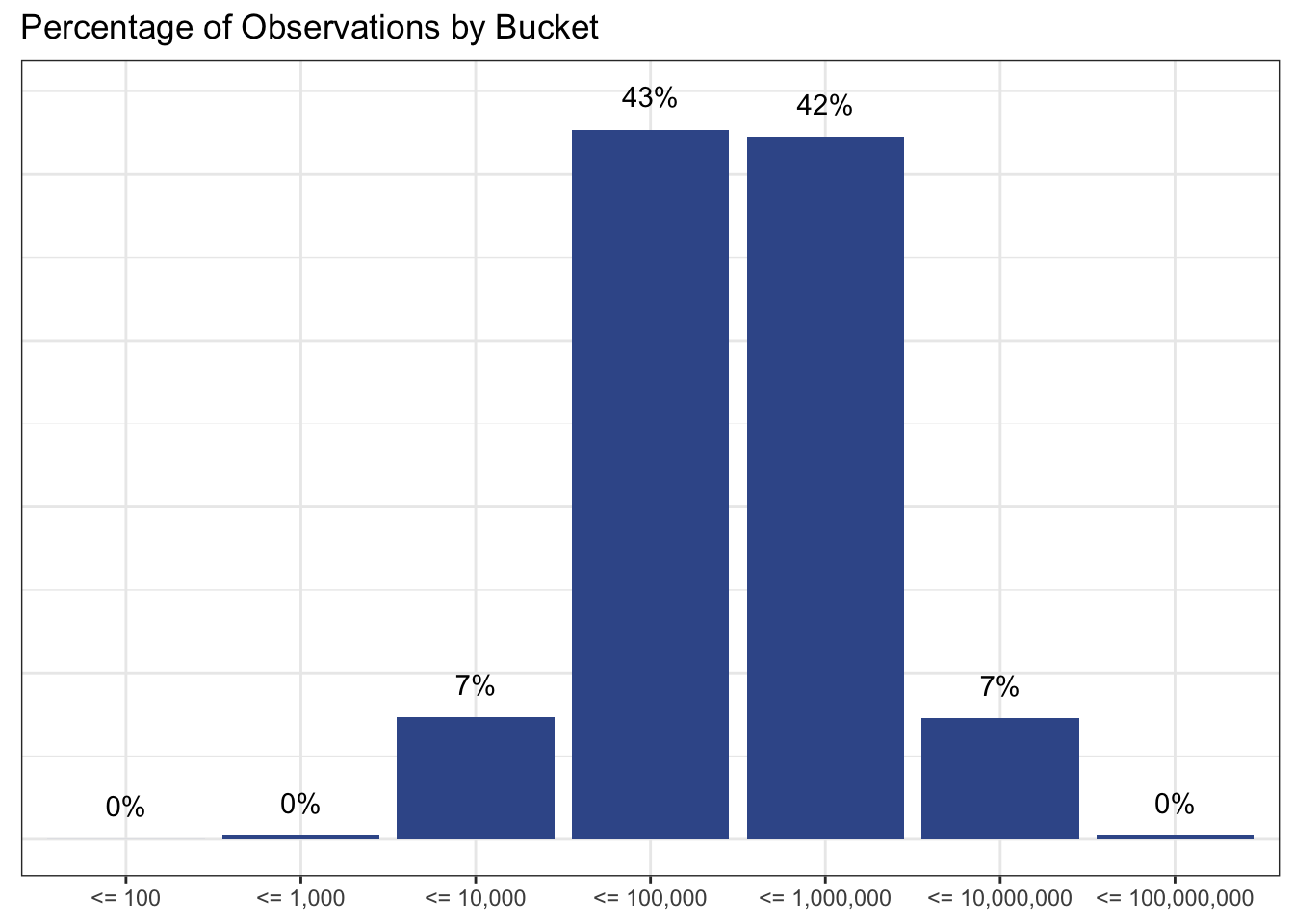
## 6 731740.292 <= 1,000,000

Let’s see how many imps are in each bucket

bucketed <- impressions %>% 
  dplyr::group_by(bucket) %>% 
  dplyr::summarise(
    imps = sum(as.numeric(imps), na.rm=T)
    , observations = n()
  ) %>%
  dplyr::ungroup() %>% 
  dplyr::mutate(
    pct_imps = imps / sum(imps)
    , pct_observations = observations / sum(observations)
    , imps = imps
  ) %>%
  dplyr::arrange(bucket)

library( DT)

DT::datatable(bucketed, options = list(dom='t')) %>% 
  formatCurrency('imps',currency='',digits=0) %>% 
  formatPercentage(c('pct_imps','pct_observations'))

Then get a promotion by making it pretty

ggplot(
  bucketed
  , aes(x=bucket, y = pct_imps)
) +
  geom_col(fill='#ed4956') +
  geom_text(aes(label=scales::percent(pct_imps, accuracy = 1)), nudge_y = 0.02) +
  theme_bw() +
  theme(axis.title = element_blank(), axis.text.y = element_blank(), axis.ticks.y = element_blank()) +
  labs( title='Percentage of Imps by Bucket') +
  scale_y_continuous(labels=scales::percent)

ggplot(
  bucketed
  , aes(x=bucket, y = pct_observations)
) +
  geom_col(fill='#3b5998') +
  geom_text(aes(label=scales::percent(pct_observations, accuracy = 1)), nudge_y = 0.02) +
  theme_bw() +
  theme(axis.title = element_blank(), axis.text.y = element_blank(), axis.ticks.y = element_blank()) +
  labs( title='Percentage of Observations by Bucket') +
  scale_y_continuous(labels=scales::percent)